Discrete and Microstrip Coupler Design - Chapter 7

Discrete and Microstrip Coupler Design

PathWave Advanced Design System (ADS)

Objective

Design a lumped element and distributed branch line coupler at 2 GHz and simulate the performance using PathWave Advanced Design System (ADS).

Background

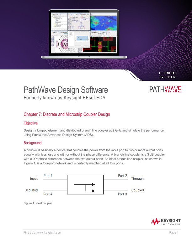
A coupler is a device that couples the power from the input port to two or more output ports equally with less loss and with or without the phase difference. A branch line coupler is a 3 dB coupler with a 90º-phase difference between the two output ports. An ideal branch line coupler, as shown in Figure 1, is a four-port network and is perfectly matched at all four ports.

The power entering port 1 is evenly divided between ports 2 and 3, with a phase shift of 90 degree between the ports. The 4th port is the isolated port and no power flows through it. The branch line coupler has a high degree of symmetry and allows any of the four ports to be used as the input port. The output ports are on the opposite side of the input port and the isolated port is on the same side of the input port. This symmetry is reflected in the S matrix, as each row can be the transposition of the first row.

The major advantage of this coupler is easier realization and the disadvantages are lesser bandwidth due to the use of a quarter wavelength transmission line for realization and discontinuities occurring at the junction. To circumvent the above disadvantages, cascading multiple sections of the branch line coupler can increase the bandwidth by a decade and a 10º – 20º increase in length of the shunt arm can compensate for the power loss due to discontinuity effects.

Objective

Design a lumped element and distributed branch line coupler at 2 GHz and simulate the performance using ADS.

Schematic Simulation Steps

1. Open the Schematic window of PathWave ADS.

2. From the lumped components library, select the appropriate components necessary for the lumped model. Click the necessary components and place them on the schematic window of PathWave ADS, as shown in Figure 3.

3. Setup an S-Parameter simulation for 1.5 GHz to 2.5 GHz with 101 points and run the simulation.

Results

Figure 4 shows about 3 dB loss through each of the output ports at the operating frequency of 2 GHz. This aligns with expectations, as -3 dB corresponds to half power, which means that the power is being split equally between the output ports. Figure 5 shows that there is very little power going into port 4 at the design frequency, which is the isolation port. Figure 6 shows that there is very little reflection happening into each of the ports at the design frequency.

Design of Distributed Branch Line Coupler

The basic steps to create a distributed model for the branch line coupler is as follows:

1. Select appropriate values for the design of the coupler. For this example, we will select following dielectric parameters:

•  Er = 4.6
•  Height = 1.6 mm
•  Loss Tangent = 0.0023
•  Metal Thickness = 0.035 mm
•  Metal Conductivity = 5.8E7 S/m

2. Calculate the wavelength λg from the given frequency specifications as follows: λg = c√ϵr f

Where,

c is the velocity of light in air

f is the frequency of operation of the coupler

εr is the dielectric constant of the substrate

3. Synthesize the physical parameters (length and width) for the λ/4 lines with impedances of Z0 and Z0/√2 (Z0 is the characteristic impedance of the microstrip line which is taken as 50 Ω).

Results

Figure 10 shows about a 3.1 dB loss through port 2 at the design frequency, whereas there is about a 4 dB loss through port 3. Figure 11 shows that output through the isolation port and Figure 12 shows the reflection parameters for all ports. These parameters are fairly low. However, these parameters reach their minimum below the design frequency by about 150 MHz.

The discrepancies between these figures and their counterparts from the lumped element model should be examined. The electromagnetic simulation from the distributed element accounts for parasitic effects, which could include loss through the materials, edge effects, and coupling between the output ports. Additionally, the distributed element design has extra length due to the added microstrip tees, which were not shown in the geometry shown in Figure 7. To compensate, the lengths of the transmission lines could be adjusted.